Macro Economics part 5
In Macro Economics Part 5 we will learn about aggregate demand and aggregate supply an it’s basic concept and its effects in National Income of macro economics

Aggregate Demand In Macro Economics part5 is the total demand for final goods and services in an economy during an accounting year.
Aggregate demand is aggregate expenditure on ex-ante (planned) consumption and ex-ante (planned) investment that all sectors of the economy are willing to incur at each income level.
In terms of Keynes, aggregate demand is the total amount of money, which the buyers are ready to spend on purchase of goods and services, produced in an economy during a given period.
It should be kept in mind that Keynes measured aggregate demand not in terms of physical goods and services but as a part of total income that society is ready to spend.
Components of aggregate demand in Macro Economics part5
(i) Private (or Household) consumption demand. The total expenditure incurred by all the households of the country on their personal consumption is known as private consumption expenditure.
Consumption demand depends mainly on disposable income and propensity to consume.
(ii) Private investment demand is the demand for capital goods by private investors. It is addition to the existing stock of real capital assets such as machines, tools, factory – building etc.
Investments demand depends upon marginal efficiency of capital (Marginal efficiency of investment) and interest rate.
Investment is of two types,
Autonomous Investment and Induced investment, but in Keynes theory investment is assumed to be Autonomous.
The basic difference between Induced Investment and Autonomous Investment
(iii) Government demand for goods and services Its curve is upward sloping rises up to Right.
In a modern economy, the government is an important buyer of goods and services.
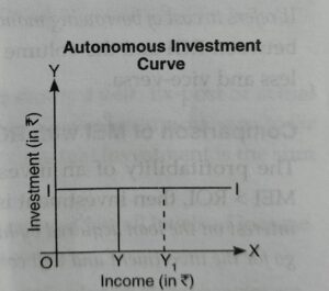
It is income inelastic, i.e., it is not affected by change in income level. The volume of autonomous investment is the same at all levels of income.
Its curve is a straight line parallel to horizontal axis.
The government demand may be on account of public needs for roads, schools, hospitals, power, irrigation etc, for the maintenance of law and order and for defense.
(iv) Demand for net export (X – M)
Net export represents foreign demand for goods and services produced by an economy.
When exports exceed imports, net exports is positive and when imports exceed, net exports is negative.
Exports and imports of a country are influenced by a number of factors such as foreign trade policy, exchange- rate, prices and quality of goods etc.
Thus, aggregate demand consists of these four types of demand.
However, for the sake of simplicity Keynes included only two types of demand,
Consumption demand (C) Investment demand (I)
Aggregate demand can be explained with the help of AD schedule and AD curve. AD= C + I
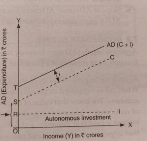
Income(Y) Consumption (C) Investment (I) AD=C+I
0 40 20 60
100 120 20 140
200 200 20 220
300 280 20 300
400 360 20 380
500 440 20 460
600 520 20 540
2. Aggregate Supply in Macro Economics pat5
The concept of aggregate supply (ΔS) is related with the total supply of goods and services by all the producers in an economy.
Four factor of production like land, labour, capital and enterprise are required for the production of goods and services.
Producers pay rent to land, wages and salaries to labour, interest to capital and Profits to the entrepreneur for their services in production.
This payment is factor- cost from producer’s point of view and factor-income from factor-owner angle.
Aggregate supply is the total amount of money value of goods and services, (which is paid to the factor of production against their factor services) that all the producers are willing to supply in an economy.
In other words, it is the total cost of production of goods and services produced in a country or it is the value of net national product at factor cost (NNPFC).
Thus, the main components of aggregate supply are: i) National Income Y ii) Consumption C iii) Saving S
National Income = Consumption + Saving==> Y=C+S
Saving (S) Consumption (C) Saving (S) AS=C+S
0 40 -40 0
100 120 -20 100
200 200 0 200
300 280 20 300
400 360 40 400
500 440 60 500
Consumption function in Macro Economics Part 5 expresses functional relationship between aggregate consumption and national income.
Thus, consumption (C) is a function of income (Y). C = F (Y)
Where, C = Consumption; F = Function; Y = Disposable income Consumption at a point of time can be measured with the equation:
C=ƒ(Y) C= Consumption , Y= National Income F= functional relationship
According to Keynes, as income increases consumption expenditure also increases but increase in consumption is smaller than the increase in income.
In other words, consumption lags behind income. This is called Keynes’ Psychological law of Consumption. According to Keynes, propensity to consume of the people remains stable in the short period.
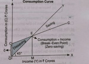
Break-even point in Macro Economics Part5 is the point in the level of income at which consumption is just equal to income. In other words, whole of income is spent on consumption and there is no saving. Below this level of income, consumption is greater than income but above this level, income is greater than consumption.
Income(I) Consumption (C)
0 40 dissaving
100 120 ”
200 200 break even point
300 280 saving
400 360 ”
500 440 ”
In the given imaginary household schedule of consumption and saving, at annual income level of Rs.200 consumption is Rs.200 and in consequence there is no saving. This is break-even point.
It is evident from the table and diagram that:2
As the income increases, consumption also increases, but the increase in consumption remains less than the increase in income.
Income can be zero but consumption can never be zero in the economy.
When C > Y, saving are negative.
When C = Y, savings are zero. This is known as break-even point. This is shown by point E in the diagram. Thus break-even point indicates a point where consumption becomes equal to income or consumption curve cuts the income curve.
Propensity to consume in Macro Economics Part5
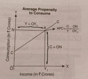
a)Average propensity to consume (APC)
The ratio of aggregate consumption expenditure to aggregate income is known , as average propensity to consume. It indicates the percentage (or ratio) of income which is being spent on consumption.
It is worked out by dividing total consumption expenditure (C) by total income (Y). Average Propensity to Consume (APC) APC= aggregate Consumption ÷ total Income
It can be explained with the help of following schedule and diagram:
Income (Y) Consumption (C) APC= C÷I
0 40 —
100 120 120÷ 100= 1.20
200 200 200÷200= 1
300 280 280÷300 = .933
Important Points for APC:
When APC is more than 1: When APC is more than 1, consumption is more than national income, i.e. before the break-even point.
APC = 1: When APC is equal to 1, consumption is equal to national income, which is known as to be break-even point.
When APC is less than 1: When consumption is less than national income, i.e. beyond the break-even point.
(b) Marginal Propensity to consume (MPC) in Macro Economics Part 5
The ratio of change in consumption (C) to change in income (Y) is known as marginal propensity to consume. It indicates the proportion of additional income that is being spent on consumption.
MPC= Change in Consumption÷ Change in Income
MPC= ΔC÷ΔY
It can be explained with the help of following schedule and diagram:
Income (Y) Consumption (C) ΔC ΔY MPC= ΔC÷ΔY
0 40 – – –
100 120 80 100 80/100= .8
200 200 80 100 80/100=.8
300 280 80 100 80/100=.8
Important points for MPC:
Value of MPC varies between 0 and 1: As we know that increase in income is either spent on consumption or saved for future use.
MPC falls with the successive increase in income: It happens because as an economy becomes richer, it has the tendency to consume smaller percentage of each increment to its income.
Propensity to save Macro Economics Part5 (or saving function)shows the functional relationship between aggregate savings and income.
S= ƒ(Y) S= Saving Y= National Income ƒ= Function relation
It is evident from the saving-function schedule and diagram that as income increases saving also increases.
Saving can be both negative and positive. Prior to break-even point saving is negative, at break-even point saving is zero and after the break-even point saving is positive.
Income (Y) Consumption (C) Saving (S=Y-C)
0 40 -40 dissaving
100 120 -20 ”
200 200 0 break even point
300 280 20 saving
400 360 40 ”
500 440 60 ”
600 520 80 ”
Important points for Saving function: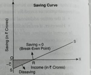
Starting Point of Saving Curve: Saving curve (SS) starts from point starts on the Y-axis, indicating that there is negative saving. (equal to amount of autonomous consumption) when national income is zero.
The saving curve will have a negative intercept on Y-axis of the same magnitude as the consumption curve has positive intercept on the Y-axis.
It happens because if consumption is positive at zero level of income, then there would be dis-savings of the same magnitude.
Break-even point .(S = 0)
Saving curve crosses the X-axis at point R which is known as break-even point as at this point saving is zero (or consumption is equal to income).
Positive Saving: After the break-even point saving is positive.
Types of propensity to save
Average propensity to save (APS): The ratio of aggregate saving to aggregate income is known as average propensity to save (APS). By dividing aggregate saving by aggregate income, we get APS.
APS= Saving (S)÷Income (Y)
Income (Y) Saving (S) APS= S/I
o -40 —
100 -20 -20/100= -.2
200 0 0/100 =0
300 20 20/300 = .067
400 40 40/400 = .1
Important Points for APS:
APS can never be 1 or more than one. As saving can never be equal to or more than national income.
APS can be 0: APS is 0 when income is equal to consumption i.e., saving = 0. This point is known as break-even point.
APS can be negative or less than 1.
At income levels which are lower than the break-even point APS can be negative as there will be dis-savings in the economy.
APS rises with increase in income. APS rises with the increase in income because the proportion of income saved keeps on increasing.
Marginal Propensity to Save :It is the ratio of change in saving (ΔS) to change in income (ΔY) is called MPS. It is proportion of income saved out of additional (incremental) income.
MPS = Change in saving ÷ Change in Income
Income(Y) Saving(S) ΔS ΔY MPS= ΔS/ΔY
It is to be noted MPS lies between 0 to 1 when ΔC=0 than MPS=1
RELATION BETWEEN APC &APS
We know that National Income is the sum of Consumption and saving Y= C+S ——– (1)
divide Income (Y) to the equation (1)
Y/Y = C/Y+S/Y
1 = C/Y + S/Y since APC= C/Y APS= S/Y
1 = APC +APS
RELATION BETWEEN MPC & MPS
As we know that sum of MPC and MPS is one
Change in Income = Change consumption +Change investment
ΔY = ΔC +ΔS ——–1
divide equation 1 by ΔY
ΔY/ΔY = ΔC/ΔY + ΔS/ΔY
1 = MPC + MPS
National Income Determination and Multiplier in Macro Economics Part 5
Determination of equilibrium level of national income in Macro Economics Part5
It refers to that point which has come to be established under the given condition of aggregate demand and aggregate supply, and has tendency to stick to that level under this given condition:
Condition to get equilibrium level of National Income
AD = AS
Investment = Saving
AD = AS
C + I = C + S
I = C + S – C
I = S
Due to some disturbance, they divert from their position, then the economic forces will work in such a manner so it drive back to the original position,
aggregate demand is equal to aggregate supply.
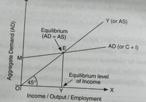
Any movement from that point would be unstable. In short, it is a position of rest. It can be explained with the help of following schedule and diagram: FIG
where aggregate supply = aggregate demand. Corresponding to point E, we derive the point E1, where saving = investment.
Determination of equilibrium level of National Income in Macro Economics Part5
Aggregate demand-Aggregate Supply Approach
It refers to the point that has come to be established under the given condition of aggregate demand and aggregate supply, and has tendency to stick to that level under this given condition where Aggregate Demand = Aggregate Supply.
Y C S I AD=C+I AS=C+S Remarks
0 40 -40 40 80 0 AD>AS
100 120 -20 40 160 100 AD>AS
200 200 0 40 240 200 AD>AS
400 360 40 40 400 400 AD=AS
500 440 60 40 480 500 AD<AS
If due to some disturbance, we divert from that position, the economic forces will work in such a manner so as to drive us back to the original position, i.e., aggregate demand is equal to aggregate supply.
In the above mentioned figure, at point P, income = consumption, which is known as to be a break-even point.
The equilibrium level of national income is attained at point E, where aggregate demand = aggregate supply.
If due to some disturbance we divert from our position, like when AD > AS , then, production will have to be increased to meet the excess demand. Consequently, national income will increase.
As we know positive relationship exists between national income and consumption, so consumption will increase, which will thereby increase the aggregate demand till we reach the equilibrium.
As against it, when AD < AS , then there would be stockpiling and producers will produce less. National income will fall and as a result consumption will start falling, which will thereby fall the aggregate demand till we reach the equilibrium.
Ex-ante saving and ex-ante investment in Macro Economics Part5:
In an economy what we plan (or intend or desire) to save during a particular period is called ex-ante saving. Against it, what we plan (or intend or desire) to invest during a particular period is called ex-ante investment.
Ex-post saving and ex-post investment.
In an economy what we actually save or what is left after deducting consumption expenditure from income is called ex-post (or realized) saving. we actually invest or what we actually add to the physical assets of an economy is called ex-post (or realized) investment
Determination of equilibrium level of National Income in Macro Economics Part 5
Saving-Investment Approach
It is the point that has come to be established under the given condition of aggregate demand and aggregate supply, and has tendency to stick to that level under this given condition where Aggregate Demand (AD)= Aggregate Supply (AS). AD = AS
Consumption (C) + Investment (I) = Consumption (C) + Saving (S)
I = S
If due to some disturbance, we divert from that position, the economic forces will work in such a manner so as to drive us back to the original position, i.e., Saving is equal to Investment.
Income(Y) Consumption(C) Saving (S) Invesrment (I) Remark
0 40 -40 40 S<I
100 120 -20 40 S<I
200 200 0 40 S<I
400 360 40 40 S=I
500 440 60 40 S>I
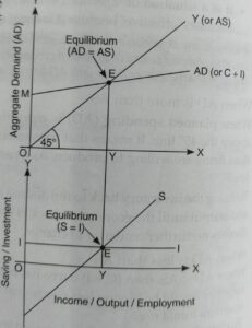
In the above figure, the equilibrium level of national income is attained at point E, where saving = investment which is derived from a point where AD = AS.
If due to some disturbance we divert from our position like when investment > saving [at Y2], then production will have to be increased to meet the excess demand.
Consequently, national income will increase leading to rise in saving until saving becomes equal to investment.
It is here that equilibrium level of income is established because what the savers intend to save becomes equal to what the investors intend to invest.
As against it, when saving > investment , then there would be stockpiling and producers will produce less.
National income will fall and as a result saving will start falling until it becomes equal to investment. It is here the equilibrium level of income is derived.
Effective Demand The level at which the economy is in equilibrium, i.e., where aggregate demand = aggregate supply, is called effective demand.
Elements of Investment in Macro Economics
INDUCED INVESTMENT : It is the investment which depends on the profit expectations and is directly is influenced by income level . It is income elastic i.e. it increase with the increase in income and vice-versa. 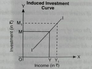
AUTONOMOUS INVESTMENT is the investment which is not affected by changes in the level of income and is not induced solely by profit motives. It is income inelastic which is not influenced by change in income .
A private investor’s demand for investment depends on two things:
The rate of return on investment or M.E.I: The expected rate of return from additional unit of investment is called marginal efficiency of investment (M.E.I).
It is defined as the expected rate of return of an additional unit of capital goods. M.E.I is very important factor in determining the investment demand. M.E.I. is determined by two factors.
Supply Price: The cost of replacing the machine under consideration with a brand new machine is known its supply price.
For example, if a machine of Rs.1 lakh is replaced in place of old machine, then Rs. 1 lakh is the supply price.
Prospective Yields: It refers to expected net returns(of all costs) from the capital asset over its lifetime.
For example, if the given machine is expected to yield revenue of Rs. 20,000 and running expenditure is Rs.2000, the prospective yield will be, 20000 – 12000 = 8000.
The Market Rate of Interest:
It refers to cost of funds borrowed for financing the investment. There exists inverse relationship between rate of interest and investment demand. Higher interest implies lower level of investment demand.
(c) Decision whether to invest or not
The investor goes on making additional investments until M.E.I becomes equal to the rate of interest.
If M.E.I is greater than the rate of interest, the investors has to increase the investment and if the rate is higher than the M.E.I, no investment is to be made.
For example,
If an entrepreneur has to pay 15% market rate of interest on the loan taken by him and he expected rate of profit i.e., M.E.I. is 30%, then he will surely go for the investment and will continue making investment till M.E.I. = Rate of Interest (ROI).
Investment demand function in Macro Economics :
Investment demand function is the relationship between rate of interest and investment demand.
There exists inverse relationship between rate of interest and investment demand. Higher interest implies lower level of investment demand.
Investment Multiplier in Macro Economics part 5
Meaning:
The ratio of change in national income (ΔY) due to a change in investment (ΔI) is known as multiplier
M. Multiplier = change in national income/ change in investment
K =ΔY/ΔI = 1/ MPS = 1/1- MPC
Excess Demand and Concepts in Macro Economics part 5
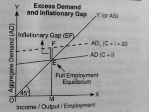
1. Excess Demand and Inflationary Gap:
When in an economy, aggregate demand exceeds “aggregate supply at full employment level”, the demand is said to be an excess demand.
Inflationary gap is the gap showing excess of current aggregate demand over ‘aggregate supply at the level of full employment’. It is called inflationary because it leads to inflation (continuous rise in prices).
A simple example :
Let us suppose that an imaginary economy by employing all its available resources can produce 2000 quintals of rice.
If aggregate demand of rice is say 10,000 quintals, this demand will be called an excess demand, because aggregate supply at level of full employment of resources is only 2,000 quintals and the result of the gap of 8000 quintals will be called as inflationary gap.
In the below diagram Inflationary gap is EF because at Full employment aggregate demand MF and aggregate supply ME.
Reasons for excess demand in Macro Economics part 5:
The main reasons for excess demand are apparently the increase in the following components of aggregate demand:
Increase in household consumption demand due to rise in propensity to consume.
Increase in private investment demand because of rise in credit facilities.
Increase in public (government) expenditure. Increase in export demand.
Increase in money supply or increase in disposable income.
Impacts of excess demand in Macro Economics part 5
Effect on General Price Level: Excess demand gives a rise to general price level because it arises when aggregate demand is more than aggregate supply at a full employment level. There is inflation in economy showing inflationary gap.
Effect on Output: Excess demand has no effect on the level of output. Economy is at full employment level and there is no idle capacity in the economy. Hence output can’t increase.
Effect on Employment: There will be no change in the level of employment also. The economy is already operating at full employment equilibrium, and hence, there is no unemployment.
Measures to control the excess demand in Macro Economics part 5:
We can control the excess demand with the help of the following policy:
(a) Monetary Policy (b) Fiscal Policy
(a) Monetary Policy: Monetary policy is the policy of the central bank of a country to control money supply and availability of credit in the economy. The central bank can take the following steps:
General Tools of Monetary Policy:
These are the instruments of monetary policy that affect overall supply of money/credit in the economy.
These instruments do not direct or restrict the flow of credit to some specific sectors of the economy. They are as under
• Bank Rate or Discount Rate (Increase in Bank Rate)
Bank rate is the rate of interest at which central bank lends to commercial banks without any collateral (security for purpose of loan).
The thing, which has to be remembered, is that central bank lends to commercial banks and not to general public.
In a situation of excess demand leading to inflation. Central bank raises bank rate that discourages commercial banks in borrowing from central bank as it will increase the cost of borrowing of commercial bank.
It forces the commercial banks to increase their lending rates, which discourages borrowers from taking loans, which discourages investment.
Again high rate of interest induces households to increase their savings by restricting expenditure on consumption.
Thus, expenditure on investment and consumption is reduced, which will control the excess demand.
• Repo Rate (Increase in Repo Rate):
Repo rate is the rate at which commercial banks borrow money from the central bank for short period by selling their financial securities to the central bank.
Reverse Repo Rate (Increase in Reverse Repo Rate):
It is the rate at which the central bank (RBI) borrows money from commercial bank.
In a situation of excess demand leading to inflation, Reverse repo rate is increased, it encourages the commercial bank to park their funds with the central bank to earn higher return on idle cash.
It decreases the lending capability of commercial banks, which controls excess demand.
Open Market Operations (OMO) (Sale of securities):
It consists of buying and selling of government securities and bonds in the open market by central bank.
In a situation of excess demand leading to inflation, central bank sells government securities and bonds to commercial bank.
With the sale of these securities, the power of commercial bank of giving loans decreases, which will control excess demand.
Increase in Varying Reserve Requirements or Legal Reserve Ratio:
Banks are obliged to maintain reserves with the central bank, which is known as legal reserve ratio. It has two components. One is the Cash Reserve Ratio or CRR and the other is the SLR or Statutory Liquidity Ratio.
Cash Reserve Ratio (Increase in CRR):
In the macro economics it refers to the minimum percentage of a bank’s total deposits, which
it is required to keep with the central bank. Commercial banks have to keep with the central bank a certain percentage of their deposits in the form of cash reserves as a matter of law.
For example, if the minimum reserve ratio is 10% and total deposits of a certain bank is Rs.100 crore, it will have to keep Rs.10 crore with the central bank.
In a situation of excess demand leading to inflation, cash reserve ratio (CRR) is raised to 20 per cent, the bank will have to keep Rs.20 crore with the central bank, which will reduce the cash resources of commercial bank and reducing credit availability in the economy, which will control excess demand.
Statutory Liquidity Ratio (Increase SLR):
It refers to minimum percentage of net total demand and time liabilities, which commercial banks are required to maintain with themselves.
In a situation of excess demand leading to inflation, the central bank increases statutory liquidity ratio (SLR), which will reduce the cash resources of commercial bank and reducing credit availability in the economy.
Selective Tools of Monetary Policy: These instruments are used to regulate the direction of credit. They are as under:
(i) Imposing margin requirement on secured loans (Increase):
Business and traders get credit from commercial bank against the security of their goods.
Bank never gives credit equal to the full value of the security. It always pays less value than the security.
So, the difference between the value of security and value of loan is called marginal requirement.
In a situation of excess demand leading to inflation, central bank raises marginal requirements. This discourages borrowing because it makes people get less credit against their securities.
(ii) Moral Suasion:
Moral suasion implies persuasion, request, informal suggestion, advice and appeal by the central banks to commercial banks to cooperate with general monetary policy of the central bank.
In a situation of excess demand leading to inflation, it appeals for credit contraction.
(iii) Selective Credit Control (SCC) [Introduce Credit Rationing]:
In a situation of excess demand leading to inflation, the central bank introduces rationing of credit in order to prevent excessive flow of credit, particularly for speculative activities. It helps to wipe off the excess demand.
(b) Fiscal Policy: The expenditure and revenue policy taken by the general government to accomplish the desired goals is known as fiscal policy. A general government can take the following steps:
(a) Revenue Policy (Increase Taxes):
(i) Revenue policy is expressed in terms of taxes.
(ii) During inflation the government impose higher amount of taxes causing the decrease in purchasing power of the people.
(iii) It is so because to control excess demand we have to reduce the amount of liquidity from the economy.
(b) Expenditure Policy (Reduces Expenditure):
(i) Government has to invest huge amount on public works like roads, buildings, irrigation works, etc.
(ii) During inflation, government should curtail (reduce) its expenditure on public works like roads, buildings, irrigation works thereby reducing the money income of the people and their demand for goods and services.
(c) Increase in Public Borrowing/Public Debt:
(i) This measure means that government should raise loans from public and hence borrowing decreases the purchasing power of people by leaving them with lesser amount of money.
(ii) So, government should resort to more public borrowing during excessive demand.
(iii) Government should make long term debts more attractive so that public may use their excess liquidity amount of money in purchasing these bonds, which will reduce the liquidity amount of money in the economy and thereby inflation could be controlled
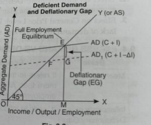
Deficient Demand or Deflationary Gap
When in an economy, aggregate demand falls short of aggregate supply at full employment level, the demand is said to be a deficient demand.
Deflationary gap is the gap showing Demand deficient of current aggregate demand over ‘aggregate supply at the level of full employment’. It is called deflationary because it leads to deflation (continuous fall in prices).
Let us suppose that an imaginary economy by employing all its available resources can produce 20,000 quintals of rice.
If aggregate demand of rice is, say 18000 quintals, this demand will be called a deficient demand and the gap of 2000 quintals will be called as deflationary gap.
Clearly here equilibrium between AD and AS is at a point less than level of full employment.
Keynes called it an under employment equilibrium.
Reasons or causes for deficient demand in Macro Economics 5
The main reasons for deficient demand are apparently the decrease in four components of aggregate demand
Decrease in household consumption demand due to fall in propensity to consume.
Decrease in private investment demand because of fall in credit facilities. Decrease in public (government) expenditure.
Decrease in export demand. Decrease in money supply or decrease in disposable income.
Impacts of deficient demand in Macro Economics 5:
Effect on General Price Level: Deficient demand causes the general price level to fall because it arises when aggregate demand is less than aggregate supply at full employment level.
There is deflation in an economy showing deflationary gap.
Effect on Employment: Due to deficient demand, investment level is reduced, which causes involuntary unemployment in the economy due to fall in the planned output.
Effect on Output: Low level of investment and employment implies low level of output.
Measures to Control the deficient demand:
(a) Monetary policy (b) Fiscal policy
Monetary Policy: Monetary policy is the policy of the central bank of a country of controlling money supply and availability of credit in the economy.
The central bank takes the following steps:
Monetary Policy: These are the instruments of monetary policy that affect overall supply of money/credit in the economy. These instruments do not direct or restrict the flow of credit to some specific sectors of the economy. They are as under:
• Bank Rate or Discount Rate (Decrease in Bank Rate):
Bank rate is the rate of interest at which central bank lends to commercial banks without any collateral (security for purpose of loan).
The thing, which has to be remembered, is that central bank lends to commercial banks and not to general public.
In a situation of deficient demand leading to deflation,
Central bank decreases bank rate that encourages commercial banks in borrowing from central bank as it will decrease the cost of borrowing of commercial bank.
Decrease in bank rate makes commercial bank to decrease their lending rates, which encourages borrowers from taking loans, which encourages investment.
Again low rate of interest induces households to decrease their savings by increasing expenditure on consumption.
Thus, expenditure on investment and consumption increase, which will control the deficient demand.
• Repo Rate (Decrease Repo Rate):
Repo rate is the rate at which commercial banks borrow money from the central bank for short period by selling their financial securities to the central bank.
In a situation of deficient demand leading to deflation, Central bank decreases Repo rate that encourages commercial banks in borrowing from central bank as it will decrease the cost of borrowing of commercial bank.
Decrease in Repo rate makes commercial banks to decrease their lending rates, which encourages borrowers from taking loans, which encourages investment.
Again low rate of interest induces households to decrease their savings by increasing expenditure on consumption.
Thus, expenditure on investment and consumption increase, which will control the deficient demand.
• Reverse Repo Rate (Decrease Reverse Repo Rate):
It is the rate at which the central bank (RBI) borrows money from commercial bank. In a situation of deficient demand leading to deflation, Reverse repo rate is decreased.
It discourages the commercial bank to park their funds with the central bank. It increases the lending capability of commercial banks, which controls deficient demand.
• Open Market Operation (Purchase of Securities):
It consists of buying and selling of government securities and bonds in the open market by central bank.
In a situation of deficient demand leading to deflation, central bank purchases government securities and bonds from commercial bank.
With the purchase of these securities, the power of commercial bank of giving loans increases, which will control deficient demand.
• Decrease in Varying Reserve Requirements:
Banks are obliged to maintain reserves with the central bank, which is known as legal reserve ratio.
It has two components. One is the Cash Reserve Ratio or CRR and the other is the SLR or Statutory Liquidity Ratio.
Cash Reserve Ratio (Decrease):
It refers to the minimum percentage of a bank’s total deposits, which is required to keep with the central bank.
Commercial banks have to keep with the central bank a certain percentage of their deposits in the form of cash reserves as a matter of law.
In a situation of deficient demand leading to deflation, cash reserve ratio (CRR) falls to 5 per cent, the bank will have to keep Rs. 5 crore with the central bank, which will increase the cash resources of commercial bank and increasing credit availability in the economy, which will control deficient demand.
The Statutory Liquidity Ratio (SLR) (Increase):
It refers to minimum percentage of net total demand and time liabilities, which commercial banks are required to maintain with themselves.
In a situation of deficient demand leading to deflation, the central bank decreases statutory liquidity ratio (SLR), which will increase the cash resources of commercial bank and increases credit availability in the economy.
Qualitative Instruments or Selective Tools of Monetary Policy: These instruments are used to regulate the direction of credit.
They are as under:
Imposing margin requirement on secured loans( Decrease): Business and traders get credit from commercial bank against the security of their goods. Bank never gives credit equal to the full value of the security. It always pays less value than the security. So, the difference between the value of security and value of loan is called marginal requirement. In a situation of deficient demand leading to deflation, central bank decreases marginal requirements. This encourages borrowing because it makes people get more credit against their securities.
• Moral Suasion:
Moral suasion implies persuasion, request, informal suggestion, advice and appeal by the central banks to commercial banks to cooperate with general monetary policy of the central bank.
In a situation of deficient demand leading to deflation, it appeals for credit expansion.
• Selective Credit Controls (SCCs):
In this method the central bank can give directions to the commercial banks not to give credit for certain purposes or to give more credit for particular purposes or to the priority sectors.
In a situation of deficient demand leading to deflation, the central bank withdraws rationing of credit and make efforts to encourage credit.
Fiscal Policy: The expenditure and revenue policy taken by the general government to accomplish the desired goals is known as fiscal policy. A general government has to take the following steps:
(a) Revenue Policy (Decrease in Taxes):
(i) Revenue policy is expressed in terms of taxes.
(ii) During deflation the government will impose lower amount of taxes so that purchasing power of the people be increased.
(iii) It is so because to control deficient demand we have to increase the amount of liquidity in the economy.
(b) Expenditure Policy (Increase in Expenditure):
(i) Government has to invest huge amount on public works like roads, buildings, irrigation works, etc.
(ii) During deflation government should increase its expenditure on public works like roads, buildings, irrigation works thereby increasing the money income of the people and their demand for goods and services.
(c) Decrease in Public Borrowing / Public Debt:
(i) At the time of deficient demand public borrowing should be reduced.
(ii) People will have more money and more purchasing power.
(iii) In brief, during period of deficient demand government should adopt the pricing of deficit budget.
(iv) Old taken debts from public should be finished and paid back to increase money in the market.
Types of Employment in Macro Economics part 5
Full employment equilibrium refers to the situation where aggregate demand is equal to aggregate supply, and all those who are able to work and willing to work (at the existing wage rate) are getting work.
Full employment doesn’t means that there is no unemployment in an economy. Unemployment also exists at full employment level because of voluntary unemployment.
unemployment in Macro Economics part5:
(i) Voluntary unemployment refers to the situation when a person is unemployed because he is not willing to work at the existing wage rate, even when work is available.
(ii) Suppose, if the market wage rate for MBA in the industries is Rs.8,000 a month, but
some of the qualified MBA’s refuse to accept job at Rs.8,000 a month, they will be considered as voluntarily unemployed.
Involuntary unemployment:
(i) Involuntary unemployment refers to a situation in which all able and willing persons to work at exist wages but do not find any work.
After reading Macro Economics part 5, you can able to understand Marco Economics basics concept aggregate demand and supply along with inflation and deflation concept in right way.
Read more :Macro Economics Part 4