Microeconomics, is study of the behaviour of individual, economic agents in the markets.For different goods and services and it try to figures out how prices and quantities of goods and services are determined through the interaction of individuals demand and supply in the markets, In this we study the consumer’s equilibrium, producer’s equilibrium, price theory, Untility analysis etc. Some of the important questions that are studied in microeconomics are as follows
How the price of a goods is determined in a market? How consumers equilibrium will be determined? What will be the level of production of a producer? How producers will be in equilibrium in perfectly competitive market? etc.
In macroeconomics, we try to get an understanding of the economy as a whole In this we focus our attention on aggregate measure such astotal output, employment and aggregate price level.
In Macro we are interested in finding out how the levels of these aggregate measures are determined and how the levels of these aggregate measures change over time. Some of the important questions that are studied in macroeconomics are as follows: What is the level of total output in the economy? How is the total output determined? How does the total output grow over time? Are the resources of the economy(eg labour) fully employed? What are the reasons behind the unemployment of resources? Why do prices rise?
An economy is a system that helps to produce good and services and enables people to earn their living. Economic problem is the problem of making the choice An economy is a system that helps to produce good and services and enables people to earn their living.
Economic problem is the problem of making the choice of scarce resources for satisfying unlimited human wants
Causes of economic problems are :
(a) Unlimited Human Wants
(b) Scarcity of Economic Resources
(c) Alternative uses of Resource
As we know that each society has unlimited wants and limited resources that have alternative uses also so every economic agent has to face the problem of allocation of resources. Every economy faces the problem of allocating the scarce resources to the production of different possible goods and services and of distributing the produced goods and services among the individuals within the economy.
The allocation of scarce resources and the distribution of the final goods and services and choice of technique are the central problems of any economy.
Following three are the central problems
(i) What to produce and in what quantities?: Every society must decide on how much of each of the many possible goods and services it will produce. Whether to produce more of food, clothing, housing or to have more of luxury goods. Whether to have more agricultural goods or to have industrial products and services. Whether to use more resources in education and health or to use more resources in building military services. Whether to have more of basic education or more of higher education. Whether to have more of consumption goods or to have
investment goods (like machine) which will boost production and consumption tomorrow.
(ii) How are these goods produced? : Every society has to decide on how much of which of the resources to use in the production of each of the different goods and services. Whether to use more labour (labour intensive technique) or
more machines (capital intensive technique). Which of the available technologies to adopt in the production
of each of the goods and services.
(iii) For whom are these goods produced?: Who gets how much of the goods that are produced in for whom are these goods produced? Who gets how much of the goods that are produced in the economy? How should the produce of the economy be distributed among the individuals in the economy? Who gets more and who gets less? Whether or not to ensure a minimum amount of consumption for everyone in the economy. Whether or not elementary education and basic health services should be available freely for everyone in the economy
Opportunity cost of a given resource can be defined as the value of the next best use to which that resource could be put.
Production possibility frontier: shows all possible combinations oftwo goods that an economy can produce with given resources and available technology, assuming that all resources are fully and efficiently utilised as shown in Fig. points K, L and M. Point H is beyond the capacity of production Any point below the PPF shows that Resources are eithe Any point below the PPF shows that Resources are either under employed or employed in wasteful manners as point G.
in Fig.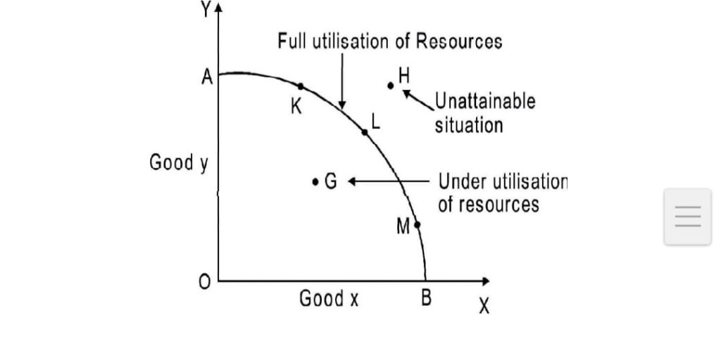
Economising of resources means use of resources in best possible manner.
Features of Production Possibility Frontier : a)It Slopes downward from left to right because to increase the
production of one good, some units of other good has to be sacrificed.(b) Concave to the origin because of increasing Marginal Opportunity Cost (MOC) or Marginal Rate of Transformation(MRT). MRT is increasing because all resources are not equally efficient in the production of both goods.
Different type of shift of PPC
Rightward shift in the PPF indicates the increase in resources or improvement in technology in case of both the
goods
Fig. 1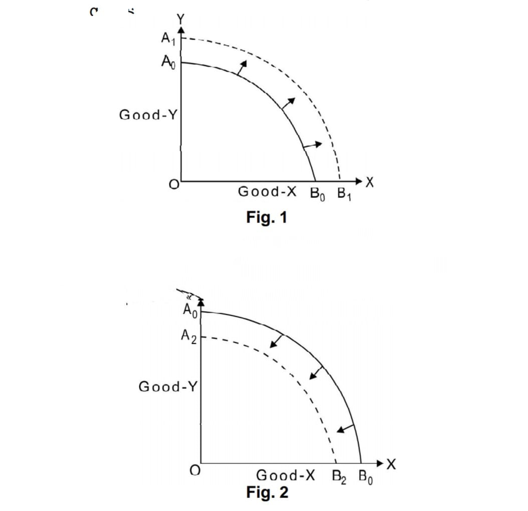
Leftward shift of PPF indicates decrease in resources oLeftward shift of PPF indicates decrease in resources or
degradation in technology in case of both the goods
Rightward/Leftward shift in PPF when no change in quantity of good Y and only change in quantity of good X.
Fig. 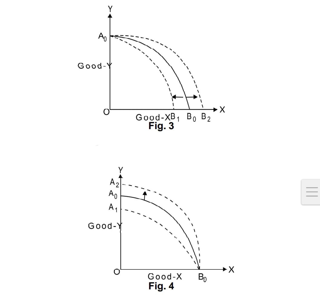
Upward/Downward shift in PPF when no change in quantity oUpward/Downward shift in PPF when no change in quantity of good Y and change only in good X.
Fig. 4
Upwards/Downward shift in PPF when no change in Quantity good X andchange only in Good Y.
PPC will shift rightwards due to all those reasons which enhances production potential, quantity and efficiency of resources in an economy.
Rightwards shift a) Increase in Resources . b) Improvement in technology c) Skill Development d) Education for all
Left ward shift a) Decrease in resource b) obsolete use of technology c). Natural Calamities (Flood, d) low standard of education
Marginal Rate of Transformation (MRT) is the ratio of number of units of a good sacrificed to increase one more unit of the other
good
MRT can also called Marginal Opportunity Cost. It is defined as the additional cost in terms of number of units of a good sacrificed to produce an additional unit of the other good.
Slope of PPF depends on MRT/MOC. i)When MOC increases, PPF is concave to origin. ii)When MOC decreases PPF is convex to origin.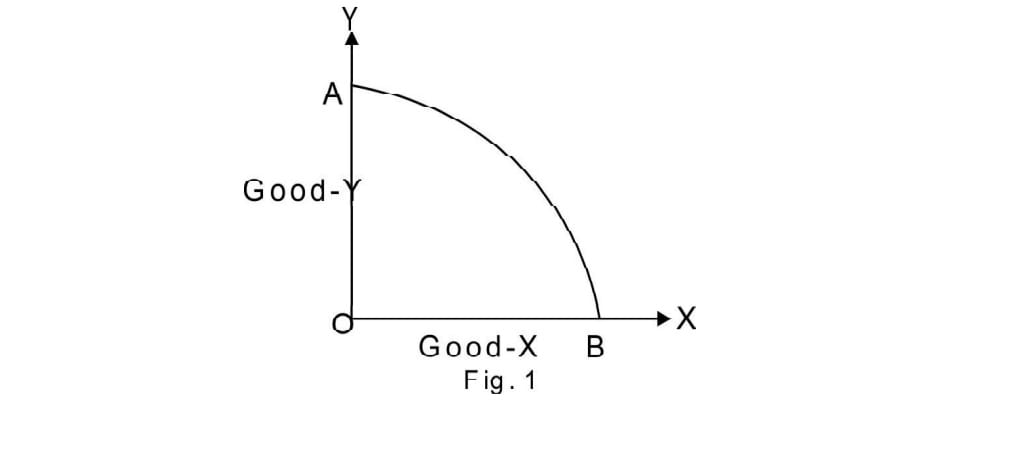
iii) When MOC remains constant, PPF is downward sloping straight line.
The slope of PPC depends on MRT/MOC In General MOC/MRT is increases therefore the PPC is concave to the origin as shown in Fig1 If MOC is constant the PPC will be a straight line and downward
sloping as shown in Fig. 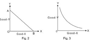
If MOC is Decreasing the PPC will be convex to the origin as shown in Fig. 3.
Positive Economics: In positive Economics analysis (i) we study how the different Mechanisms functions.(ii) It deals with the things in the Actual “as they are”(iii) It studies the facts which can be verified. Examples India is over populated; prices are Rising in India.
Normative Economic
(i) In normative Economics we try to understand whether the different Mechanism are desirable or not.
(ii) It deals with the idealistic situation instead of actual situation.
(iii) It studies the statements about facts that can’t be verified.
Example we should control the over population. Prices should not Rise etc.
Consumer Equilibrium
Introduction
This chapter consists of Utility, Law of Diminishing Marginal Utility, Budget line, Budget Constraint, Monotonic Preferences, Indifference Curve, Consumer Equilibrium in Cardinal (single and several Commodities) and Ordinal (indifference curve) Approaches.
Utility
Utility is the power or capacity of a commodity to satisfy human wants. in other words, utility of a commodity means the amount of satisfaction that a person gets from consumption of a good or service.
There are two kinds of Utility:
Cardinal Utility Approach (Marginal Utility)
The satisfaction the consumer derives by consuming goods and services can be measured with a number. Cardinal utility is measured in terms of utils (the units on a scale of utility or satisfaction).
According to cardinal utility the goods and services that are able to derive a higher level of satisfaction to a consumer will be given higher utils and goods that result in a lower level of satisfaction will be assigned lower utils.
Cardinal utility is a quantitative method that is used to measure consumption satisfaction.
Ordinal utility Approach (Indifference Curve Analysis or J.R. Hicks analysis):
It states that the satisfaction the consumer derives from the consumption of goods and services cannot be measured in numbers. It uses a ranking system in which a rank is provided to the satisfaction that is derived from consumption.
Ordinal utility, the goods and services that offer a customer a higher level of satisfaction will be assigned higher ranks and the goods and services that offer a lower level of satisfaction will be assigned lower ranks. It is a qualitative method that is used to measure consumption satisfaction.
Cardinal Utility
Total utility is the total satisfaction a consumer obtains from consuming a given amount of a particular good. Alternatively, total utility is the sum of marginal utilities obtained from consumption of successive units of a commodity. It is measured in utils.
TU = MU1 + MU2 + MU3 +—— MUn= sum value ofM
Marginal utility is the additional utility derived from consumption of an additional unit of a commodity. MU= TUn+1 – TUn
Law of diminishing marginal utility states that marginal utility derived from the consumption of a commodity declines as more units of that commodity are consumed.
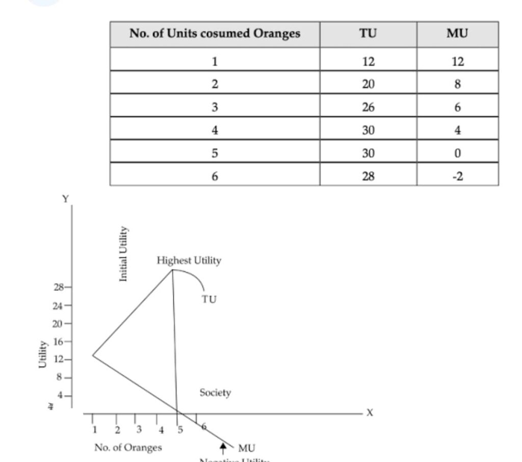
It’s can be seen from the above schedule that total utility increases at a diminishing rate when marginal utility falls.
Law of diminishing marginal utility will operate only when consumption is a continuous process. For example, if one apples is consumed in the morning and another in the afternoon, the second apples may provide equal or higher satisfaction as compared to the first one.
Law of diminishing marginal utility will not be applied with regard to education/ knowledge because every effort to get education/ knowledge increases the utility.
6. Relationship between marginal utility and total utility:
- When MU decreases, TU increases at a diminishing rate. (As shown in graph till consumption level OQ).
- When MU is zero, TU is constant and maximum at P.
- When MU is negative, TU starts diminishing.
Consumer Equilibrium Under Marginal Utility Analysis (Cardinal Approach)
1. Consumer’s Equilibrium is a situation where a consumer gets maximum satisfaction out of his given money income and given market price.
2. Consumer’s equilibrium through utility analysis can be explained in two ways
a)A single commodity b) Two or several commodities
(a) Single Commodity Consumer Equilibrium:
(i) When a consumer purchases a unit of a commodity, a consumer compares its price with the expected utility from it. Utility obtained is the benefit, and the price payable is the cost. The consumer compares benefit and the cost. He will buy the unit of a commodity only if the benefit is greater than or at least equal to the cost.
(ii) Equilibrium Conditions for Single Commodity Consumer Equilibrium
Necessary Condition Let us suppose, MU of one rupee refers to the utility obtained from the purchase of commodities with one rupee. The marginal utility of a product in terms of money should be equal to its price. Marginal utility is equal to price, i.e. MU = Price.
If MU > Price, a rational consumer, keeps on going to purchase an additional unit of a commodity as long as MU = Price. MU > Price implies when benefit is greater than cost and whenever benefit is greater than cost a consumer keeps on consuming additional unit of a commodity till MU = Price. It is so because according to the law of diminishing marginal utility, MU falls as more is purchased. As MU falls, it is bound to become equal to the price at some point of purchase.
If MU< Price being a rational consumer he would have to reduce the consumption of a commodity as long as MU=Price. MU < Price implies when benefit is less than cost and whenever benefit is less than cost, consumer keeps on decreasing the additional unit of a commodity till MU = Price. It is so because according to the law of diminishing marginal utility, MU rises as less units are consumed. As MU rises, it is bound to become equal to the price at some point of purchase.
Sufficient Condition: Total gain falls as more is purchased after equilibrium. It means that consumer continues to purchase so long as total gain is increasing or at least constant.
It can be explained with the help of the following schedule and diagram:
Suppose, the price of commodity X in the market is Rs.10 per unit. It means he has to pay Rs.10 per unit. Suppose, the utility obtained from the first unit is 14utils (= Rs.10). The consumer will buy this unit because the utility of this unit is greater than the price. Whether the consumer consumes second unit or not depends on the utility obtained from the second unit. Suppose, it is 12utils (= Rs.10). He will buy the second unit also. Again, suppose the utility of the third unit is 10utils (= Rs.10). here the price of commodity becomes equal to marginal utility. If the consumer goes for the 4 unit in which he gets Mu of Rs 8 The price paid is also Rs.10. Since the utility not equals to price he will not buy the fourth unit also. Consumer will not buy the fifth unit because utility of this unit is 6 utils (= Rs.10) which is less than the price. It is not worth buying the fourth unit. The consumer will restrict his purchase to only 3 units.
The difference between utility and price of a unit of a commodity represents the gain to the consumer from that unit. For example, utility of first unit of X is Rs.14 and price paid is Rs.10 The gain is Rs.4 . Similarly, gain from the second unit is 2 total gain(4 +2+0). Marginal Gain from the 5th unit is negative, i.e. -4 . The consumer maximises gain when he buys only 3 units.
The conclusion is that in a single commodity case a consumer makes purchases only upto the point where MU = Price.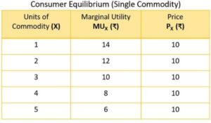
In the below diagram, consumption (demand) is recorded on the horizontal axis and marginal utility (price) is recorded on the vertical axis.The price is and MUfalls as consumption increases at E MU =Price 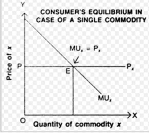
MU > Price . As MU is greater than the price, it means benefit is greater than the cost. It will induce the consumer to buy more units of the goods. In fact, the consumer must buy to reach equilibrium again. It shows that when price of goods falls, its demand rises and the consumer will continue to buy more units until MU falls enough to be equal to the price again.
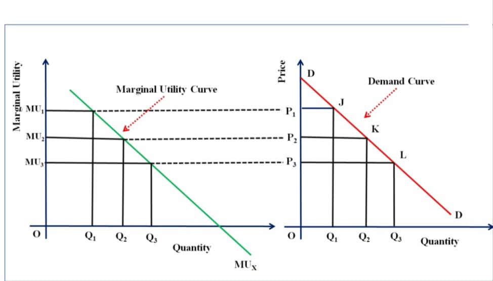
As we consume Q1 , Q2,Q3 quantity it marginal utility falls that is due to fall in the price the demand of the commodity increases as the price fall MU becomes gater and consumers consumes more
(b) Two Commodities Consumer Equilibrium (Law of Equi-Marginal Utility or Law of Substitution or Gossen’s Second Law or Law of Maximum Satisfaction)
The law of diminishing marginal utility is applicable in this case the law of equi- marginal utility /law of maximum satisfaction / Gossen’s Second law which states that a consumers get maximum satisfaction when ratio of MU of two commodities and their respective prices are equal .
Suppose there are two commodities Xand Y upon which the consumer wants to allocate his income to attain the equilibrium The consumer will be in the equilibrium when the MU of both the commodities will be equal to the respective prices
Two necessary conditions i) MUx/Px= MUy/Py = MUm
Marginal utility of last rupee spent on each commodity is same.
Expenditure on commodity X+Expenditure on commodity Y=Money Income.
ii), Marginal utility falls as more and more units of a commodity are consumed.
we get MUx, MUy X is more than marginal utility from the last rupee spent on commodity Y. So, to attain the equilibrium consumer must increase the quantity of X, which decrease the MUx and decrease the quantity of Y which will increase the MUy. Increase in quantity of X and decrease in quantity of Y continue till commodity X is less than marginal futility from the last rupee spent on commodity Y. So, to attain the equilibrium the consumer must decrease the quantity of X, which will increase the MUx and increase the quantity of Y, which will decrease the MU . Decrease in quantity of X and increase in quantity of Y continues till MUx=MUy .
the consumer will spend all his income on one commodity, which is highly unrealistic.
This can also be explained with the help of the following numerical example and diagram:
Let us suppose that the total money of the consumer is Rs 7 which he wants to spent on both the commodities x and y . The price of each of these commodities is Rs1 /unit than a consumer can purchase either of x or y In the below diagram and schedule MU of X is represented by OY and MU of Y by O1Y1 . MUx and MUy are the marginal utility of the respected commodities.
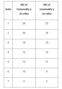
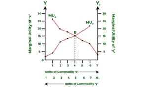
The first rupee is spent to purchase x , 2nd rupee on y , 3rd rupee on x , further on y ,again on x and so on until Rupees 7 are consumed which will give maximum satisfaction in this combination From the above table and figure, it is obvious that the consumer will spend the first rupee (shown in brackets)
The Consumer Budget
Let us consider a consumer who has only a fixed amount of money (income) to spend on two goods the prices of which are given in the market. The consumer cannot buy any and every combination of the two goods that she may want to consume. The consumption bundles that are available to the consumer depend on the prices of the two goods and the income of the consumer. Given her fixed income and the prices of the two goods, the consumer can afford to buy only those bundles which cost her less than or equal to her income.
Budget Line
(a) Budget line is a graphical representation which shows all the possible combinations of the two goods that a consumer can buy with the given income and prices of commodities. It is also called consumption possibility line.
(b) Suppose, a consumer has Rs. 600 as his money income and decides to spend this entire income on the purchase of two commodities X1 and X2 where per unit price of X1 be Rs. 100 and that of X2 Rs.50 per unit and these prices remain unchanged during the period in which the consumer buys these commodities.
(c) If the consumer decides to spend his entire money income of Rs. 600 on the purchase of commodity Xx, he can buy 6 units of X, and on purchase of X2 i. e., 12 units of X2 (shown in given figure as point p and V).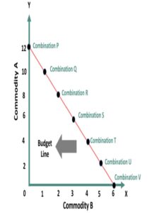
Points P and v are two extreme possibilities of the combination of that the can purchase with his given money income and prices of commodities. By joining points P and V we can know all the possible combinations of two commodities X1and X2, which can be purchased with Rs.600. We, therefore get the budget line VP. It is also called Price income line. Thus, the budget line is the set of bundles that costs exactly M.
(d) The equation of budget line is:
P1 X1+ P2 X2 = M …(1)
Where, P1 and P2 are the prices of two commodities:
X1 and X2 are the quantities of two commodities P1 X1 is the expenditure on commodity X1
P2 X2 is the expenditure of on commodity X2
(e) Budget constraint shows the combination of two commodities whose expenditure can be less than or equal to money income. So, there is possibility of saving.
P1 X1 + P2 X2 < M
(f) Budget set is the collection of all bundles of pieces of goods that a consumer can buy with his income at the prevailing market prices.
(g) Market rate of Exchange is the rate at which market requires to sacrifice one commodity to gain an additional unit of another commodity is called market rate of exchange.
Change in Quantity of Good Sacrificed (P1 X1 ) Change in Quantity of Good Gained (P2 X2)
Price of Good Gained [P1 ] Price of Good Sacrificed [P2
Preferences Of The Consumer (Ordinal Utility Analysis)
1. Ordinal Utility states that the satisfaction the consumer derived from the consumption of goods and services cannot be measured in numbers.
2. Rather, ordinal utility uses a ranking system in which a rank is provided to the satisfaction that is derived from consumption.
Consumer’s preferences are assumed to be such that between any two bundles (x1,x2) and (y1,y2), if (x1,x2) has more of at least one of the good and no less of the other good as compared to (y1,y2), the consumer prefers (x1,x2) to (y1,y2). Preferences of this kind are called monotonic preferences.
Thus, a consumer’s preferences are monotonic if and only if between any two bundles the consumer prefers the bundle which has more at least one of the pieces of good and no less of the other
Equilibrium in Ordinal (indifference curve) Approaches.
INDIFFERENCE CURVE This curve shows different combination of two goods and each combination offering the same level of satisfaction of the consumer.
The graph as 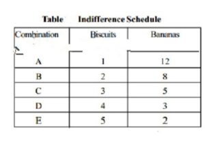
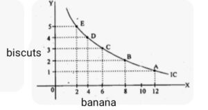
The main properties of Indifference curve i) It has a negative slope / downward slope which shows that more of one commodity implies less of the other, so that total satisfaction remain same ii) Indifference curves are convex to origin point because of diminishing the marginal rate of substitution it means that every additional unit of good a consumer is willing to give up lesser and lesser amount of another good iii)Indifference curve touches neither of axis because it is assumed that consumer buys a combination of two goods If it touches the axis it means that one commodity is consumed and consumption of other is zero iv) It never touches or intersect the other indifference curve that represent of different level of satisfaction and the law of transitivity does not hold to be true.
Indifference Set are those combinations of two goods which offer the consumer the same level of satisfaction and the consumer is indifferent across any number of combination in his indifferent sets
Monotonic Preference means that greater consumption of the commodity by the consumer gives him higher level of satisfaction.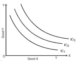
Indifference map refers to the set of indifference curves corresponding to different levels of the consumers fig given .Higher the indifference curve higher shall be the level of satisfaction
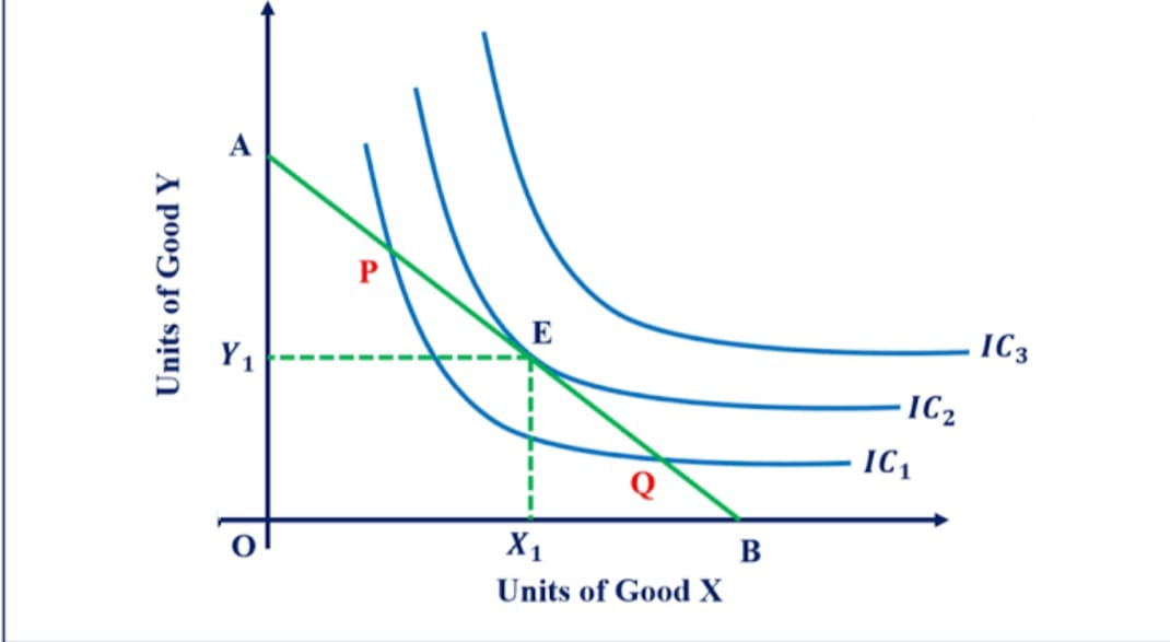
According to indifference curve analysis the consumer is at the point where the slope of indifference curve is equal to the slope of budget line / price line . The two main conditions i)MRSxy= Px/Py ii) At the point of equilibrium , Indifference curve is convex to origin. It implies that at the point of equilibrium MRS must be diminishing At the point P the equilibrium point at which budget line touches the IC2 which is with the consumer budget but IC3 are not affordable curve as his income does not permit. The point A could not be the point of equilibrium in this because at the point P MRSxy > Px/Py in this case the consumer will consume more of x and less of y will a result MUx falls and MUy will rise this process will continue till the time MRS = Px/Py At the lower point Q MRS<Px/Py in this consumer will demand more of good Y and less of good X MUy will and MUx will rise till MRS=Px/Py.
. Demand is a quantity of a commodity which a consumer wishes to purchase at a given level of price and during a specified period of time.
In other words, demand for a commodity refers to the desire to buy a commodity backed with sufficient purchasing power and the willingness to spend.
. Desire is just a wish for a commodity and a person can desire a commodity even if he does not have the capacity to buy it from the market whereas demand is desire backed by purchasing power that is to say whatever an individual is willing to buy from the market in a given period of time at a given price. A poor person can desire to own a car but that will not become a demand because he does not have the purchasing power to buy a car from the market.
Factors affecting personal (individual) demand:
Price of the commodity has Inverse relationship exists between price of the commodity and demand of that commodity.It means with the rise in price of the commodity the demand of that commodity falls and vice-versa.
.Price of related goods: It may be of two types:
- Substitute goods
- Complementary goods
(i) Substitute Goods: Substitute goods are those goods which can be used in place of another goods and give the same satisfaction to a consumer. There would always exist a direct relationship between the price of substitute goods and demand for given commodity.
It means with an increase in price of substitute goods, the demand for given commodity also rises and vice-versa. For example, Pepsi and Coke.
(ii) Complementary Goods: Complementary goods are those which are useless in the absence of another goods and which are demanded jointly. There would always exist an inverse relationship between price of complementary goods and demand for given commodity.
It means, with a rise in price of complementary goods, the demand for given commodity falls and vice-versa. For example pen and refill.
Income of a Consumer: There are three types of goods:
For Normal Commodity: For normal commodity, with a rise in income, the demand of the commodity also rises and vice-versa. Shortly, direct relationship exists between income of a consumer and demand of normal commodity.
For Inferior Goods: For inferior goods, with a rise in income, the demand of the commodity falls and vice-versa.
Shortly, inverse relationship exists between income of a consumer and demand of inferior goods.
For Necessity Goods: For necessity goods, whether income increases or decreases, quantity demanded remains constant.
(d) Taste and Preferences of the Consumer: Tastes, preferences and habits of a consumer also influence its demand for a commodity.
For example, if Black and White TV set goes out of fashion, its demand will fall. Similarly, a student may demand more of books and pens than utensils of his preferences and taste.
Miscellaneous: Some of the other factors affecting the demand of a consumer are: Change in weather, change in number of family members, expected change in future price, etc.
4. Market demand refers to the quantity of a commodity that all the consumers are willing and able to buy, at a particular price during a given period of time.
5. Factors affecting Market demand:
- Price of the commodity
- Price of related commodity
- Income of a consumer
- Taste and preference of a consumer
- Miscellaneous
- Population Size: Demand increases with the increase in population and decreases with the decrease in population. This is because with the increase (or decrease) in population size, the number of buyers of the product tends to increase (or decrease). Composition of population also affects demand. If composition of population changes, namely, female population increases, demand for goods meant for women will go up.
- Distribution of Income: Market demand is also influenced by change in distribution of income in the society. If income is not equally distributed, there will be less demand. If income is equally distributed, there will be more demand.
. Demand function shows the relationship between quantity demanded for a particular commodity and the factors that are influencing it.. Individual demand function refers to the functional relationship between individual demand and the factors affecting the individual demand.
Market demand function refers to the functional relationship between market demand and the factors affecting the market demand.
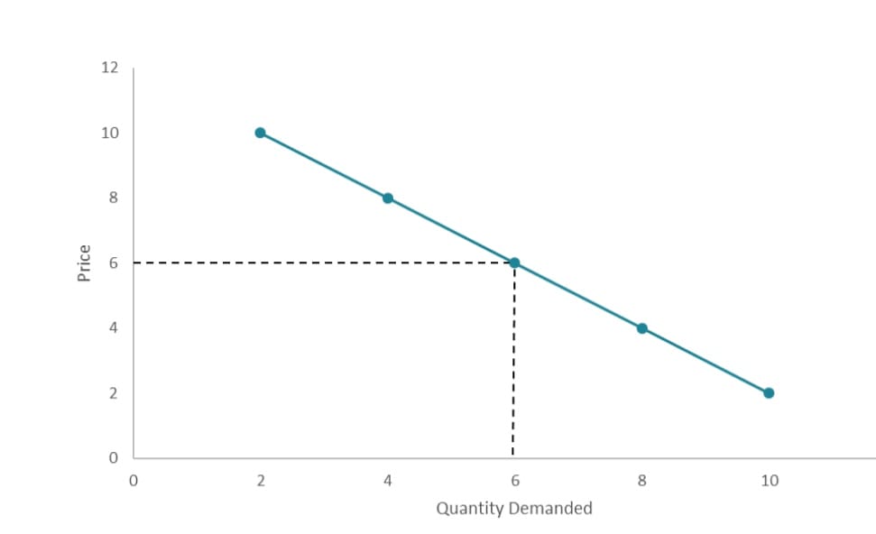
Demand Schedule is a table showing different quantities being demanded of a given commodity at various levels of price. It shows the inverse relationship between price of the commodity and its quantity demanded. It is of two types:
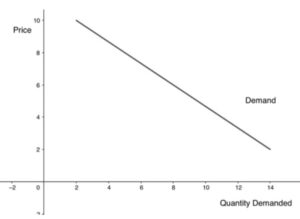
Individual Demand Schedule. Individual demand schedule refers to a table that shows various quantities of a commodity that a consumer is willing to purchase at different prices during a given period of timeIndividual Demand curve is the graphical representation drived from the individual demand schedule.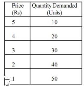
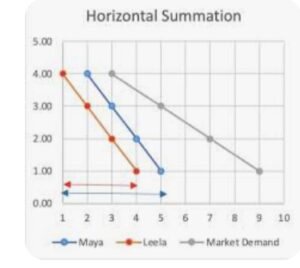
Market Demand Schedule is a tabular statement showing various quantities of a commodity that all the consumers are willing to buy at various levels of price. It is the sum of all individual demand schedules at each and every price .The graphical representation of market schedule is market demand curve. 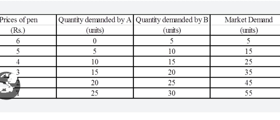
Movement Along The Demand Curve Or Change In Quantity Demanded
1. It is based on Law of Demand which states that quantity demanded of the commodity changes due to the changes in price of the commodity.
2. The change in quantity demanded due to the change in price of the commodity is known as movement along the demand curve. It may be of two types; namely,
Expansion in Demand (Increase in quantity demanded)
(b) Contraction in Demand (Decrease in quantity demanded)
3. Expansion in Demand (Increase in quantity demanded or downward movement along the demand curve):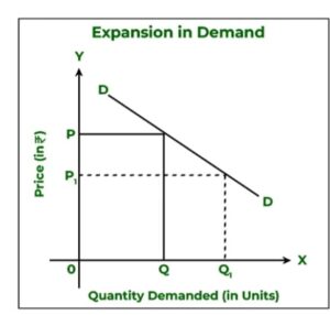
It is based on Law of demand which states that quantity demanded of the commodity rises due to the fall in price of the commodity. The rise in quantity demanded due to the fall in price of the commodity, is known as expansion in demand. It is shown in the figure given above
• In the given diagram price is measured on vertical axis whereas quantity demanded is measured on horizontal axis. A consumer is demanding OQ quantity at OP price.
• But, due to fall in price of the commodity from OP to OP1 the quantity demanded rises from OQ to OQ1 which is known as expansion in demand.
4. Contraction in Demand (Decrease in quantity demanded or upward movement
along the demand curve):
(a) It is based on Law of Demand which states that quantity demanded for the commodity falls due to the rise in price of the commodity.
(b) The fall in quantity demanded due to the rise in price of the commodity is known as contraction in demand.
(c) This is shown in the figure given below: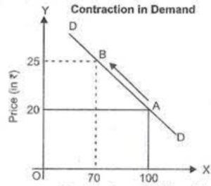
• In the given diagram, price is measured on vertical axis whereas quantity demanded is measured on horizontal axis. A consumer is demanding OQ quantity at OP price.
• But, due to rise in price of the commodity from OP to OP1, the quantity demanded falls from OQ to OQ1 which is known as Contraction in Demand.
Shift In Demand Curve Or Change In Demand
1. It is based on factor other than price. If demand changes due to the change in factors other than price, it is known as shift in demand curve.
2. It may be of two types,
(a) Increase in Demand (b) Decrease in Demand
(a) Increase in Demand:
An increase in demand means that consumers demand more at a given price of a commodity. It’s conditions are: i)Price of substitute goods rises. ii) Price of complementary goods falls.
Income of a consumer rises in case of normal goods. Income of a consumer falls in case of inferior goods. When preferences are favourable.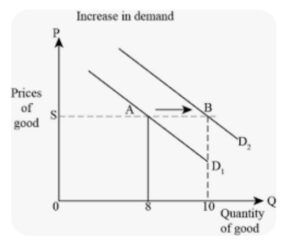
In the given diagram, price is measured on vertical axis whereas quantity demanded is measured on horizontal axis. A consumer is demand the quantity demanded rises from 8 to 10 which is known as increase in Demandwhen demand curve shifts ti D1D1 to D2D2
(b) Decrease in Demand:
A decrease in demand means that consumers demand less at a given price of a commodity.
• Price of substitute goods falls.
Price of complementary goods rises. Income of a consumer falls in case of normal goods.
Income of a consumer rises in case of inferior goods.hen a preference becomes unfavourable.
(iii) In the given diagram price is measured on vertical axis whereas quantity demanded is measured on horizontal axis. A consumer is demanding OQ quantity at an OP price.
(iv) But, due to the change in factor other than price, the demand curve shifts leftward to DD to D1D1
(v) With the leftward shift in demand curve from DD to D1D1, the quantity demanded falls from OQ to OQ1 which is known as decrease in demand.
Causes Of Law Of Demand And Exceptions To Law Of Demand
1. There is a inverse relationship between price of the commodity and quantity demanded
for that commodity which causes demand curve to slope downward from left to right.
2. It is because of the following reasons:
(a) Income effect: Quantity demanded of a commodity changes due to change in purchasing power (real income), caused by change in price of a commodity is called Income Effect.
Any change in the price of a commodity affects the purchasing power or real income of a consumers although his money income remains the same. When price of a commodity rises more consumer has to spend more on purchase of the same quantity of that commodity. Thus, rise in price of commodity leads to fall in real income, which will thereby reduce quantity demanded is known as Income effect. Its substitution of one commodity in place of another commodity when it becomes relatively cheaper.
A rise in price of the commodity let coke, also means that price of its substitute, let thumps up, has fallen in relation to that of coke, even though the price of thumps up remains unchanged. So, people will buy more of thumps up and less of coke when price of coke rises. consumers will substitute thumps up for coke. This is called Substitution effect.
Law of Diminishing Marginal Utility:
This law states that when a consumer consumes more and more units of a commodity, every additional unit of a commodity gives lesser and lesser satisfaction and marginal utility decreases.
The consumer consumes a commodity till marginal utility (benefit) he gets equals to the price (cost) they pay, i.e., where benefit = cost.
For example, a thirsty man gets the maximum satisfaction (utility) from the first glass of water. Lesser utility from the 2nd glass of water, still lesser from the 3rd glass of water and so on. Clearly, if a consumer wants to buy more units of the commodity, he would like to do so at a lower price because the utility derived from additional unit goes on decreasing
(d) Additional consumer:
When price of a commodity falls, two effects are quite possible:
New consumers, that is, consumers that were not able to afford a commodity previously, starts demanding it at a lower price.
Old consumers of the commodity starts demanding more of the same commodity by spending the same amount of money. As the result of old and new buyers push up the demand for a commodity when price falls.
3. Exceptions to the Law of Demand are:
(a) Inferior Good or Giffen Goods:
(i) Giffen goods are a special category of inferior goods in which demand for a commodity falls with a fall in its price.
(ii) In case of certain inferior goods when their prices fall, their demand may not rise because extra purchasing power (caused by fall in prices) is diverted on purchase of superior goods.
(b) Goods expected to become scarce or costly in future:
(i) These goods are purchased by the household in increased quantities even when their prices are rising upwards.
(ii) This is due to the fear of further rise in prices.
(c) Goods of Ostentation:
(i) Status symbol goods are purchased not because of their intrinsic value but because of status or prestige value.
(ii) The same jewellery when sold at a lower price sells poorly but offered at two times the price, sells quite well.
4. Necessities:
(a) The law of demand is not seen operating in case of necessities of life such as food grain, salt, matchstick, milk for children, etc.
(b) A minimum quantity of these goods has to be bought whether the prices are high or low. In such cases, law of demand fails to operate.
5. Ignorance: Being ignorant of prevailing prices, a consumer may buy more of a
commodity when its price has gone up.
6. Emergency: In times of emergency like flood, famine or war, the households do not
behave in a normal way and consequently law of demand may not operate