Statistics part 2
Statistics part 2 covers the chapter of Diagrammatic Presentation, with suitable example of Arithmetic mean, Median , Mode , Co-relation , Index Number that covers syllabus of class 11
DIGARAMATIC PRESENTATION
It is a graphical representation of data to help understanding pattern , relationship and distributions .It is the method that provides the quickest understanding of the actual situation to be explained by data comparison to tabular and textual presentation but diagrammatical presentation if data translate quite effectively the highly abstract idea contained in number in comprehensive form
The main advantages of the diagrammatic presentation are i) They are attractive , impressive ii) It is easy to remember and simplify the data iii) It saves the time because complex mass of data can be presented in very simple way in form of diagram which is easy to understand and saves lot of time iv) They are useful in making comparison and give more information with universal applicability.
Types of Diagram :
a) Simple Bar Diagram comprises of group of rectangular bars of equal width for each class of the data. In this type of diagram , one bar represents only one figure there are as many bars as the number of figures
b) Multiple Bar Diagram :It is the diagram to make comparison between two /more variables like export and import or income , expenditure Number of students in different games in successive years
c)In case of subdivided bar diagram the bar corresponding to each phenomenon is divided into carious components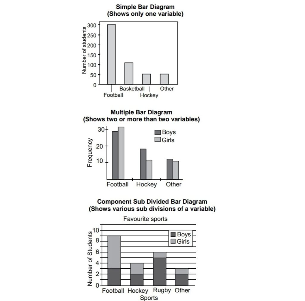
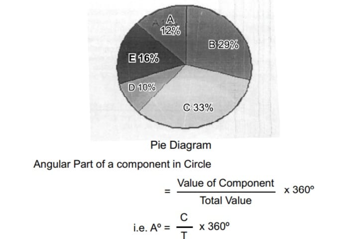
Pie Diagram : It is the chart of circular shape broken into sub – divisions. The size of the section indicates the proportion of each compound to the whole. It is a circle can also be portioned into sections to show proportions of various component
A circle in the pie diagram is irrespective of the values of radius, let 100= 360 degree one part is equal to 3.6 deg . To find the angle the component should subtend at the center of the circle ,each % figure of every component is multiplied by 3.6
Graphic Presentation of data are the two types i) Frequency diagram ii)Arithmetic/ time series diagram
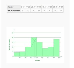
Frequency distribution graphs : The data is expressed in terms of class intervals /class limits/ mid value expressed along x axis and frequency at y axis. i) Line frequency graph it is used in discrete series where variables are measured on the x axis and frequency on y axis . ii) Histogram is the graph of frequency distribution in which class intervals are plotted along x axis and frequency on y axis It is a graphical representation of such data , height for aera of rectangle is the quotient of height is frequency and base / width is class interval It is never drawn for discrete variable data If classes are not continuous first they are converted into continuous series. 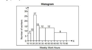 iii) Frequency Polygon used to represent frequency distribution on the graph It is plane bounded by straight line . It is alternative to histogram and also derived from histogram itself. It is suitable to histogram for studying the shape of the curve the simplest way to plot frequency polygon is to join the mid points of the top side of consecutive rectangles of histogram.
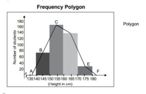 iv) Frequency Curve in which the vertices of the frequency polygon are joined by smooth by smooth curve .It is the free hand curve passing through the mid points of the tops of the rectangles of histogram It is to be noted that the curve should start from the end of the base
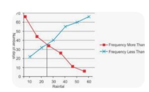
 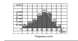 v) Ogive are the curve by representing cumulative frequency distribution on a graph. It is also called cumulative frequency curv along Y axis aganist class limits of the There are two types of cumulative frequencies for example i) Less than ii) more than according there are two is ogives for any grouped frequency distribution data. Cumulative frequencies are plotted along Y axis against class limits of the frequency distribution For less than ogive the cumulative frequency are plotted against the respective upper limits of the class intervals where as for more than ogives the cumulative frequencies are plotted against the respective lower limits of the class intervals. We can locate median graphically by putting the perpendicular on axis from the point X axis of intersection of both the ogives
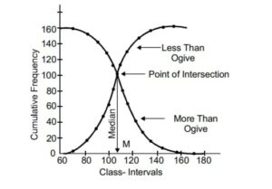
ARITHMETIC LINE GRAPH : It is also called time series graph is the method of diagrammatic presentation of data . In it time ( hour/ day/ date/ week/ month/ year etc) is plotted along along x axis and the value of the variable / the time series data along y axis . A line graph by the joining these plotted points , thus, obtained is called is time series graph .It helps to understand the trend, periodically in long term data. They are of two types a) One variable graph it is fluctuation of the said line that shows the variations in the variable and the distance of the points from the base line of graph indicates the magnitude b) Two / more variable than variable graph are shown on the same graph , then it is preferred to use different types of lines eg a dotted line , broken line or thick line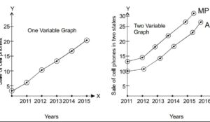
Advantages of Graphical Presentation : It is attractive and impressive , It is simple and understandable presentation on data. It is useful in comparison , location of the positional averages .There is no need for mathematically knowledge It is useful in quick comparison .
Limitation of Graphic Presentation of Data :It has limited application and misuse is possible They are subjective in nature and do not have accuracy .
Measure of central tendency : A central tendency is a single value which represents the whole mass of data.
Mean :
Arithmetic mean is the number which is obtained by
adding the values of all the items of a series and dividing the total
by the number of items.
Types of mean : It is of two kinds if mean
Simple Arithmetic mean : When all items of a series are
given equal importance then it is called simple arithmetic
mean
Weighted Arithmetic mean : When different items of a
series are given different weight with relative importance is know as weighted arithmetic mean.
Merits of mean :It is easy to calculate which is rigidly defined.
It is based on all values and easy in comparison
Demerit It is affected by the extreme values. Mean value may not exist in the series. It may lead to misleading solution
Incase of individual series :Runs scored in 10 innings are 50,59, 90,08, 106 ,117, 59 ,91, 7, 74
Arithmetic mean = sum of the runs scored/ number of innings
A.M = 661/10 = 66.1
In case of discrete series
X — | 3 | 5 | 9 | 11 |
f—- 2 6 5 3 total = 15
f.x 6 30 45 33 total = 114
mean = sum of f.x/ sum of f = 114/15= 7.6
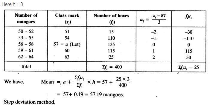
Incase of class interval series
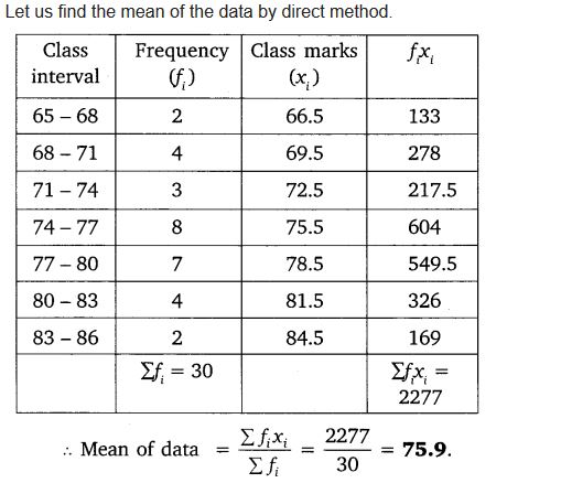 Solution:
Median – The Median is the middle value of the series which divides it into two equal parts.
Merits of Median It is easy to calculate and is not affected by the extreme values. It can be located on graph. It can be calculated even when data is incomplete.
Demerits of Median It requires organization of data but is not based on all the items and it is not suitable for algebraic treatment Affected by fluctuations of items.
Incase of individual series : Let the number be given
2,4, 5, 14, 12, 10 , 11, 7,9, 20 ,23
first of all arrange the number in ascending order such as
2, 4, 5, 7, 9, ,10, 11, 12, 14, 20,23 number of digits 11
median place value = (number of digit +1 ) /2 =( 11+1 )/2 =12/2=6
6th value in the series will be the median ie 10
incase of discrete series
X — 5 10 15 20 25 30
freq 3 5 2 6 2 3
c.f 3 8 10 16 18 21
median place value =last cf value /2 = 21/2= 10.5 this value lies at 20 so median is 20 as value till 10 lies in 15 but above it it is in 20
Median incase of class interval series
class interval| 10-20 | 20 –30 | 30- 40 | 40 -50 |
frequency 5 20 15 25
cf 5 25 40 65
median place = last frequency÷ 2= 65÷2= 32.5
the median lies in class of 30 -40
formula for median = L1 +( N/2 -c)×i/f
L1 = lower limit of median class , N = last cf value , c= cf of previous class of median class i= class difference f = frequency of median class
L1 = 30 N/2 = 32.5 c = 25 f=15 i=10
by putting the values median = 30 + (32.5 -25 ) ×10/15
median = 30 + 7.5 ×10/15 = 30 + 75/15 = 30 +5 = 35
4. Mode – Mode is the value which occurs most frequently in the series
Merits of Mode: It is easy to calculate and is not affected by the extreme values. It can be located on graph. It is the most representative value in the given series.
Demerits of Mode: It is not based on all the values and not suitable for statistical treatment. It’s method of grouping is complicated. It is an uncertain measure.
Incase of individual series
40,43, 50 , 53, 53,57,57,57,57,60,60, 60, 63,63,65,70,80
maximum number of observations is 57 (5 times )
Incase of discrete series
Size (x) 8 9 10 11 12 13 14 15
freq 5 6 8 7 18 8 9 6
highest frequency is 18 size is 12 mode is 12
Incase of class interval series :
class interval 0-5 5- 10 10-15 15-20 20-25
frequency 2 4 15 6 7
the modal class is 10-15 as it has highest frequency
formula Z= L1 + (f1-f0) ×i ÷ (2f1-f0-f2)
Z= mode L1 = lower limit of modal class = 10 fo =frequency of previous class of modal class =4 f1 = frequency of modal class =15 f2 frequency of preceding class of the modal class =6 i= class mark =5
by putting the values in the formula of mode
Z = 10 + (15 -4)×5 ÷ ( 2×15 – 4-6 )
Z= 10 + 11×5÷ (30-10 ) = 10 + 55/20 = 10 + 2.75= 12.75 mode
Differences between Arithmetic mean, median and mode
Mode = 3 Median – 2 Mean OR Z = 3M – 2X
MEASURES OF CO – RELATION :
Coefficient of co-relation is determined by dividing the sum of products of the deviation from their respective means by the product of the number of pairs and their standard deviation
r=( sum of production of deviation from their respective means)÷(number of pairs × standard deviation of both series
Karl Pearsons method :
actual mean method r = (´∑xy) ÷ ( N σx.σy )
direct method
r={ NΣxy- ∑x. ∑y } ÷[{√ N∑x²-(∑x)²}× {√N∑y²-( ∑y)²}]
step deviation / short cut method;
r=[ N∑dxdy – ∑dx ,∑dy ] ÷[ √{N∑dx² – (∑dx)²}{√N∑dy²-(∑dy)²]
Spearman ‘s rank method r = 1- (6 ∑D²) ÷ (N³ – N )
Examples 1 find the coefficient of co-relation number of x items 30 and of y are 30 SDx =3 SDy=2 and ∑xy =150
r = ∑xy÷(N σx.σy ) = 150 ÷ (30×3×2) =150 ÷(180) =0.833
Find the co-relation between x and y
X 12 15 18 21 24 27 30 total 147
X-Xm=x -9 -6 -3 0 + 3 +6 +9
x² 81 36 9 0 9 36 81 ∑x²=252
Y 6 8 10 12 14 16 18 total 84
Y-Ym =y -6 -4 -2 0 2 4 6
y² 36 16 4 0 4 16 36 ∑y² =112
x.y 54 24 6 0 6 24 54 ∑xy=168
calculation Xm =∑X÷N= 147÷7=21
Ym = ∑Y÷N = 84÷7 =12
formula r = ∑xy ÷ √∑x².∑y²= 168 /√252×112= 168/168=1
example : calculate the coefficient of co relation between the data of X and Y by assumed mean/step deviation method
X 30 32 34 35 37 38 40 42 44
taking assumed mean for x =37 dx= x-37
dx -7 -5 -3 -2 0 1 3 5 7 ∑dx= -1
Y 22 25 27 28 29 30 31 32 33
taking assumed mean for y =28 dy= Y- 28
dy -6 -3 -1 0 1 2 3 4 5 ∑dy = 5
dx² 49 25 9 4 0 1 9 25 49 ´∑dx² = 171
dy² 36 9 1 0 1 4 9 16 25´∑dy² 101
dx.dy 42 15 3 0 0 2 9 20 35
∑dx.dy =126
r= ( N∑dx.dy – ∑dx.∑dy )÷[ {√N∑dx²- (∑dx)²×{√N∑dy²(∑dy)²}]
r=[ 9×126 – (-1) (5)]÷[ √(9.171 88 – (-1)²)×√( 9.101 – (5)²)]
r =( 1134 + 5) ÷[√1538×√884 ] =1139/1166.015 =0.976
INDEX NUMBER : An index number is a statistical measure designed to show changes in magnitude of a variable or group of related variables with respect to time, geographical location or other characteristics.
Characteristics of Index Numbers :
Index numbers are not qualitative statements like prices are
rising or falling. It is a precise measurement of quantitative
changes in the concerned variable.
Index numbers show changes in terms of averages.
when it is said that price level has been increased that
does not mean that price of all goods and services have been
increased. But it means that on and average prices have been
increased.
An Index number, indicating change in magnitude, as of price,
wage, employment, or production. It is, relative to the
magnitude at a standard or base value usually taken as 100.
Types of Index Numbers
a)Price Index : It measure changes in price over a specified
period of time. It is basically the ratio of the price of a certain
number of commodities at a present year as against base
year.
Wholesale price Index (WPI),
Consumer Price Index (CPI) Or Cost of Living Index
(COLI).
b) Quantity Index : These indices pertain to measuring change in
volume of commodities like goods produced or goods
consumed E.g. Index of Industrial production (IIP)
c) Value Index : It compare changes in the monetary value of
imports, exports production or consumption of commodities.
It Base Year refer to the year of reference with which prices of
current year are compared to measure the changes
Rate of Inflation : The rate of inflation is measured as the
percentage change between price levels over a specific period
of time. Inflation is the general and ongoing rise in the level of
prices in an economy.
It is Sensex : a short form of Bombay Stock Exchange (BSE)
sensitive Index with 1978-79 as base. The value of the sensex
is with reference to this period. It is the benchmark index for the
Indian stock market
METHODS OF CONSTRUCTION PRICE INDEX :
a) Simple average method :
commodity price 2011-12 P0 price 2022-23 P1
wheat 20/kg 25/kg
Rice 30/kg 40/kg
Pluses 60/kg 80/kg
sugar 30/kg 40/kg
∑P0 = 140 ∑P1= 185
P01= ( ∑P1÷∑P0 ) %=( 185÷140)%= 1.3214×100= 132.14 it is also called price index.
price index taking base year as 2016;
year price index base (P1×100)÷ P0
2016 40 40×100/40 = 100
2017 50 50×100/40= 125
2018 60 60×100/40 = 150
2019 70 70×100/40 = 175
2020 80 80×100/40 =200
2021 90 90×100/40 = 225
2022 95 95×100/40 = 237.5
∑(P1/P0)×100 =1212.5
Price Index P01= 1212.5/7= 173.215
commodity | base year | current year |
| P0 Qo | P1 Q1 | P0Q0 | P1Q0 | P0Q1 | P1Q |
A 6 50 10 56 300 336 500 560
B 2 100 2 120 200 240 200 240
C 4 60 6 60 240 240 360 360
D 10 30 12 24 300 240 360 288
E 8 40 12 36 320 288 480 432
∑P0Qo 1360∑P0Q1=1344∑P1Q0=1900ΣP1Q1=1880
Important formula
a) Laspayre’s Method = (∑P1Q0×100)÷∑P0Q0
b) Paasche’s Method =( ∑P1Q1×100)÷ ∑P0Q1
c) Fishers Method = 100 ×√( ΣP1Q1 ×ΣP1Q0)÷√(P0Q0×P0Q1)
or price index = √laspayres price index×√ Paasches price index
100. √(1900 ×1880)÷(1360 × 1344) = 100×√1.953= 1.3974×100=139.74 as price index
Follow us on : Facebook
Follow us on : Instagram
Read More : Statistics